Economic Order Quantity (EOQ) for Spare Parts: Formula and How to Apply It in Your CMMS

Economic Order Quantity (EOQ) for spare parts is a formula that calculates the ideal order quantity that minimises total inventory costs — balancing ordering frequency against holding costs. For maintenance teams managing spare parts, applying EOQ inside a spare parts inventory software system reduces over-ordering, prevents stockouts, and cuts unnecessary warehousing costs. According to the International Data Corporation, manufacturers spend 10–20% of total maintenance budgets on inventory carrying costs — EOQ directly targets that figure.

This guide covers the EOQ formula in full, a worked example using realistic maintenance numbers, how to apply it step by step inside your CMMS, and where EOQ has limits so you know when a different approach fits better.

What Is EOQ for Spare Parts?

EOQ stands for Economic Order Quantity. It is an inventory management formula that finds the order size that produces the lowest total cost — accounting for both the cost of placing orders and the cost of holding stock. First developed by Ford W. Harris in 1913, EOQ remains one of the most practical tools in MRO inventory management because it is mathematically grounded, easy to explain to stakeholders, and directly actionable inside any CMMS with an inventory module.

In spare parts management, the core tension EOQ solves is this: ordering small quantities frequently drives up purchasing and handling costs; ordering large quantities infrequently drives up holding, storage, and obsolescence costs. EOQ finds the point where both cost curves intersect at the minimum. That intersection tells your maintenance planner exactly how many units to order each time, so the total annual cost of managing that part stays as low as possible.

EOQ is most effective for parts with predictable, steady demand — consumables like bearings, belts, filters, seals, and fasteners. It works less well for critical insurance spares or low-usage parts with erratic demand, which we address in the limitations section below.

The EOQ Formula for Spare Parts Explained

The EOQ formula is:

EOQ = √ (2DS / H)

Where:

• D = Annual demand (units consumed per year)
• S = Ordering cost per order (cost to place one purchase order, including admin, freight, and processing)
• H = Annual holding cost per unit (storage, insurance, capital tied up, and obsolescence risk per unit per year)

Breaking Down Each Variable

Getting accurate inputs is more important than understanding the math. Here is how each variable typically looks in a maintenance context.

Annual demand (D) comes directly from your CMMS work order history. Pull the consumption data for the part across the last 12 months. For a bearing that gets replaced 24 times per year across four identical pumps, D = 24. If your CMMS tracks parts consumption per asset, this number is already available in your inventory management reports.

Ordering cost (S) includes staff time to raise a purchase order, supplier processing fees, delivery charges, and receiving labour. A typical industrial operation spends $20–$80 per purchase order depending on procurement complexity. If you use a blanket purchase order arrangement with a supplier, S drops significantly — which raises the EOQ and makes larger, less frequent orders optimal.

Holding cost (H) is the annual cost to keep one unit in stock. It includes storage space allocation, insurance, the opportunity cost of capital tied up in stock, and obsolescence risk. Holding cost is typically expressed as a percentage of unit value — commonly 20–30% per year for industrial spare parts. If a bearing costs $50 and your holding cost rate is 25%, H = $12.50 per bearing per year.

EOQ Worked Example for a Maintenance Team

A maintenance team at a food processing facility manages V-belt replacements across 12 conveyor lines. Here are the inputs:

• Annual demand (D): 120 belts per year
• Ordering cost (S): $45 per purchase order
• Unit cost: $18 per belt
• Holding cost rate: 25% per year, so H = $18 × 0.25 = $4.50 per belt per year

Applying the formula:

EOQ = √ (2 × 120 × 45 / 4.50) = √ (10,800 / 4.50) = √ 2,400 = 49 belts

The team should order 49 belts per order. At 120 belts per year, that works out to approximately 2.4 orders per year — roughly one order every five months. Before applying EOQ, they were ordering 20 belts at a time (6 orders per year), which was driving unnecessary ordering costs. After switching to EOQ-based ordering and setting the reorder quantity to 49 in their CMMS, they reduced annual ordering cost from $270 to $108 while holding cost stayed nearly the same.

EOQ vs Reorder Point vs Safety Stock: When to Use Which

EOQ answers "how much to order." Two related concepts — reorder point (ROP) and safety stock — answer "when to order" and "how much buffer to keep." All three work together in a complete spare parts inventory policy, but they serve different purposes. The table below clarifies which tool does what.

In practice, your CMMS will use all three in combination. EOQ sets the order quantity. ROP triggers the order automatically when stock drops to the right level. Safety stock is added on top of ROP for critical parts where the cost of a stockout — measured in downtime tracking data — exceeds the cost of carrying extra stock.

How to Apply EOQ in Your CMMS

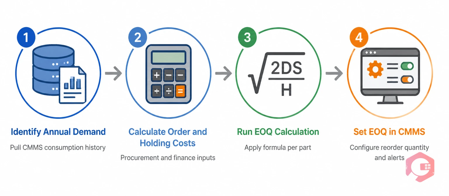
Calculating EOQ on paper is the easy part. The real value comes from encoding EOQ into your CMMS so the system enforces optimal ordering automatically — without your team needing to manually check stock levels or remember reorder quantities. Here is the four-step process.

Step 1 — Identify Annual Demand Per Part

In your CMMS, run a parts consumption report filtered to the last 12 months. For each high-usage part, record the total units consumed. Parts that appear in fewer than six work orders per year are likely candidates for min-max management rather than EOQ — the calculation is most valuable for parts consumed 20 or more times annually. Cryotos's report builder generates parts consumption reports by asset, location, or time period, giving you the demand data you need without manual spreadsheet work.

Step 2 — Calculate Ordering and Holding Costs

Work with your procurement and finance teams to establish your ordering cost per purchase order and your holding cost rate. If you do not have this data, use these starting estimates: $40–$60 per order for a standard industrial operation; 20–25% of unit value per year for holding cost. Record both figures. Even approximate values produce EOQ calculations that are significantly better than arbitrary order quantities.

Step 3 — Run the EOQ Calculation

Apply the formula for each target part. A spreadsheet with the formula =SQRT(2*D*S/H) speeds this up. Prioritise parts where you currently order very frequently (high ordering cost exposure) or very infrequently in large quantities (high holding cost exposure) — those are where EOQ will produce the biggest cost savings. For a 200-part inventory, focus first on the top 20% of parts by annual spend — ABC analysis helps identify which parts those are.

Step 4 — Set EOQ as Reorder Quantity in CMMS

With your EOQ calculated, enter the value as the reorder quantity for each part in your CMMS inventory module. Set the reorder point (ROP) based on lead time and average demand. In Cryotos, the spare parts inventory software supports minimum threshold alerts that trigger automatically when stock hits the ROP level — the system creates a work request or purchase requisition at the EOQ quantity without any manual intervention. This closes the loop between the calculation and the actual purchasing behaviour, which is where most teams lose the benefit: they calculate EOQ once but still order arbitrary quantities because the CMMS is not configured to enforce it.

EOQ Limitations for Spare Parts Management

EOQ is a powerful tool, but it rests on assumptions that do not hold for every part in a maintenance storeroom. Knowing where it breaks down prevents costly mistakes.

• Assumes constant, predictable demand: EOQ works best when a part is consumed at a steady rate throughout the year. Parts with seasonal demand spikes, unpredictable failure-driven consumption, or very low overall usage produce unreliable EOQ values. For these parts, a min-max policy or manual review cycle fits better.
• Does not account for criticality: EOQ minimises cost. It says nothing about whether running out of a part is tolerable. For critical insurance spares — a main shaft seal on a sole-source pump, for example — the consequence of a stockout vastly exceeds any holding cost. These parts need safety stock decisions driven by downtime cost analysis, not pure EOQ logic.
• Ignores supplier constraints: Suppliers often have minimum order quantities, price breaks at volume thresholds, or lead times that make your EOQ impractical. If your EOQ is 7 units but the supplier's minimum order is 24, you need to balance EOQ against those constraints rather than following the formula blindly.
• Static formula in a changing environment: EOQ assumes that demand, ordering cost, and holding cost are fixed. In reality, all three change. Equipment upgrades alter part consumption rates; carrier cost increases affect ordering cost; obsolescence risk increases as assets age. EOQ values should be recalculated at least annually, or whenever there is a significant change in any input variable. Your CMMS historical data makes this recalculation straightforward if you have been tracking parts consumption consistently.

Why Maintenance Teams Use EOQ: Key Benefits

When applied correctly, EOQ produces measurable improvements across several dimensions of maintenance operations.

• Reduces total inventory cost: By finding the balance point between ordering and holding costs, EOQ consistently produces lower total annual costs than arbitrary order quantities. Teams that move from ordering whatever fits on a pallet to EOQ-based quantities typically see 10–20% reductions in total inventory carrying costs.
• Prevents both overstock and stockouts: Overordering ties up capital and creates obsolescence risk; underordering leads to emergency orders and unplanned maintenance delays. EOQ reduces both failure modes simultaneously by anchoring order quantities to actual consumption data.
• Improves CMMS data quality: Implementing EOQ forces maintenance teams to collect accurate demand data, ordering costs, and holding costs — data that improves every other inventory decision and makes the CMMS a more reliable planning tool.
• Supports preventive maintenance reliability: When PM tasks require specific parts, EOQ-sized stock ensures those parts are consistently available without the storeroom being unnecessarily full. Preventive maintenance execution rates improve when technicians can trust that required parts are in stock when the work order is generated.
• Enables scalable inventory policies: Once EOQ is calculated for your top-consumption parts and encoded in the CMMS, the system manages reordering automatically. Maintenance planners and storeroom managers spend less time on manual stock checks and more time on higher-value planning work.

Frequently Asked Questions

What is EOQ in maintenance management?

EOQ in maintenance management is the order quantity that minimises the total annual cost of purchasing and holding a spare part. It balances the cost of placing frequent small orders against the cost of storing large quantities infrequently, using the formula EOQ = √(2DS/H), where D is annual demand, S is ordering cost per order, and H is annual holding cost per unit.

How do you calculate EOQ for spare parts?

To calculate EOQ for a spare part, you need three inputs: annual demand (units consumed per year from CMMS history), ordering cost per purchase order (admin, freight, and processing costs), and annual holding cost per unit (typically 20–25% of unit cost per year). Apply the formula EOQ = √(2DS/H). A bearing consumed 60 times per year with a $50 order cost and $5 annual holding cost gives an EOQ of √(2 × 60 × 50 / 5) = √1,200 = 35 units.

What is the difference between EOQ and reorder point?

EOQ tells you how much to order each time. Reorder point (ROP) tells you when to place the order — specifically, when stock drops to the level where a new order must be placed to avoid running out before the next delivery arrives. ROP = (average daily demand × supplier lead time) + safety stock. EOQ and ROP are complementary: you use ROP to trigger the order and EOQ to set the order size.

Does EOQ work for all types of spare parts?

EOQ works best for spare parts with consistent, predictable annual demand — consumables like belts, bearings, seals, and filters. It is less suitable for critical insurance spares held against rare failure events, parts with erratic demand patterns, or parts where the cost of a stockout significantly exceeds any holding cost savings. For those parts, safety stock calculations and criticality-based stocking policies are more appropriate.

How does a CMMS help implement EOQ?

A CMMS supports EOQ implementation by providing the demand data (parts consumption history per work order), hosting the inventory module where EOQ quantities and reorder points are stored, and triggering automatic alerts or purchase requisitions when stock hits the reorder point at the EOQ quantity. This automation means the optimal order quantity is enforced in every purchasing decision without relying on manual review.

Applying EOQ to your spare parts inventory is one of the highest-return, lowest-effort improvements a maintenance team can make to inventory management — and a CMMS makes it automatic once the calculation is done. Cryotos CMMS combines spare parts inventory management with automatic minimum-threshold alerts, parts consumption reporting, and LIFO/FIFO/Average Cost valuation — giving your team everything needed to implement and enforce EOQ-based ordering across your full storeroom. Book a free demo today and see how Cryotos can help you cut inventory carrying costs while keeping the right parts available when your team needs them.