Capacity modeling for manufacturing is the process of calculating how much good output a line or plant can really produce. A useful model starts from how equipment actually runs, using maintenance data such as breakdown frequency, repair time, and planned shutdowns instead of nameplate speed.
Many production plans fail because they assume machines run at full speed all shift. Breakdowns, PM windows, and slow running then turn every plan into a firefight. This guide shows how to build a capacity model from maintenance records, test what-if scenarios, and plan output that the shop floor can deliver. A Computerized Maintenance Management System holds most of the data you need.
Key Takeaways
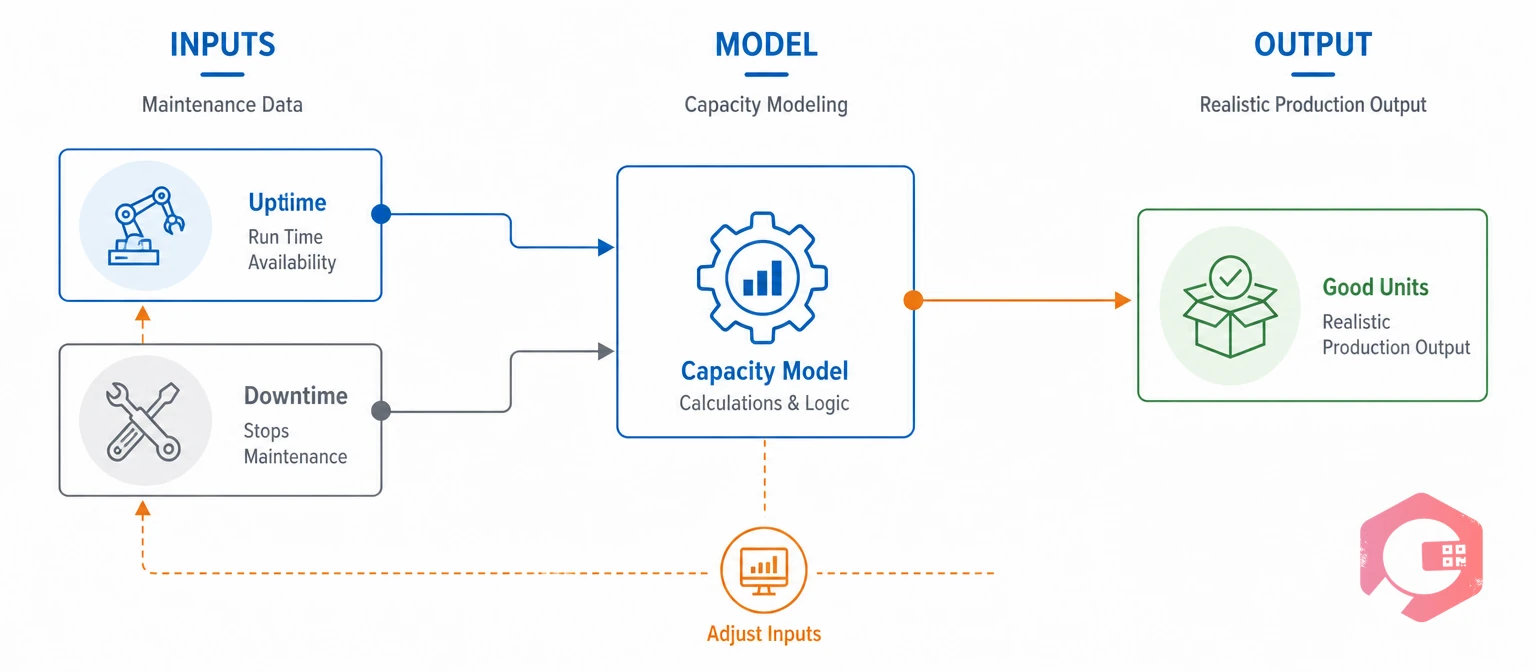
A capacity model is a set of calculations that turns available hours, run rates, and losses into expected good output. It answers simple questions. How many units can we ship this week? Which machine limits us? Which change would add the most output?
Capacity modeling is the engine behind capacity planning. The model calculates what assets can produce, and planning uses that number to set shifts, accept orders, and decide on new equipment.
Using shared definitions matters more than it seems. If two shifts count downtime differently, the model breaks before you start.
Planners often mix up these terms, and the mix-up leads to plans the shop floor cannot meet. The table shows how each one differs and where its data comes from.
| Capacity type | What it means | What reduces it | Data source |
|---|---|---|---|
| Design (nameplate) capacity | Maximum output at rated speed, 24/7 | Nothing; it is a theoretical limit | OEM specification |
| Scheduled capacity | Output possible during planned shift hours | Shift pattern, holidays, planned PM windows | Shift calendar and PM schedule |
| Effective capacity | Output expected after normal losses | Breakdowns, changeovers, speed loss, rejects | Maintenance history and OEE records |
| Actual output | Good units really produced | All of the above plus one-off events | Production records |
Plan production against effective capacity, not design capacity. The gap between the two is where maintenance can help most. Overall equipment effectiveness (OEE) is the standard way to measure that gap.
Most of the data a capacity model needs already sits in work orders and downtime logs. The key is to collect it the same way for every asset, every shift.
Inherent availability is MTBF divided by the sum of MTBF and MTTR. It shows the share of run time an asset is up before planned stops are counted. An asset with an MTBF of 45 hours and an MTTR of 3 hours is up 93.75% of its running time.
Want a quick baseline for your own assets? Use the MTBF calculator to work out time between failures before you build the model.

Capacity modeling for one line fits in a simple spreadsheet. Follow these six steps in order. Use the same time period for every input, usually one week.
Step 6 is the one most plants skip. A model that has never been checked against real output will not earn a planner's trust.
Here is a simple weekly model for one packing line. It runs two 8-hour shifts, six days a week, at a nameplate rate of 120 units per hour.
| Step | Calculation | Result | Data used |
|---|---|---|---|
| Scheduled hours | 2 shifts × 8 h × 6 days | 96 h | Shift calendar |
| Minus planned PM | 96 h − 6 h | 90 h | PM schedule |
| Availability from breakdowns | MTBF 45 h ÷ (45 h + MTTR 3 h) = 93.75% | 84.4 h run time | Work order history |
| Rate after speed loss | 120 units/h × 90% performance | 108 units/h | OEE records |
| Gross output | 84.4 h × 108 units/h | About 9,110 units | Calculated |
| Good output | 9,110 × 98% quality | About 8,930 units | Quality records |
If the planner had used the nameplate rate across all 96 hours, the plan would show 11,520 units. That is nearly 2,600 units the line cannot make. Every missed order traces back to that one assumption.
Capacity modeling pays off when you test changes before you spend money. Change one input at a time. Then compare the result with the baseline of about 8,930 good units a week.
| Scenario | What changes | Good output per week | Gain vs baseline |
|---|---|---|---|
| Baseline | Current MTBF, MTTR, PM, and speed | About 8,930 | None |
| Faster repairs | MTTR drops from 3 h to 2 h | About 9,120 | About +190 |
| Fewer minor stops | Performance rises from 90% to 95% | About 9,425 | About +495 |
| PM moved off shift | 6 h of PM done on the idle seventh day | About 9,525 | About +595 |
The biggest gain here comes from scheduling, not repair speed. Moving PM out of production hours adds three times more output than cutting MTTR by an hour. This is where capacity modeling changes decisions. Preventive maintenance software with a shared calendar makes that kind of shift easy to plan and track.
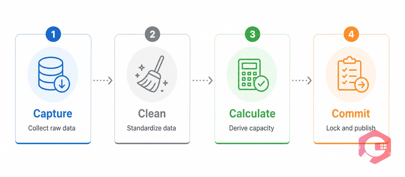
The Data-to-Capacity Ladder is a four-step method for turning maintenance records into a model planners trust. Each step depends on the one before it.
The Data-to-Capacity Ladder:
Most maintenance teams already collect the raw data for the first rung. The climb is about consistency, not new tools.
Every line has one step that limits output, and capacity modeling shows you which one it is. The theory of constraints says to protect that step first, because an hour lost there is an hour lost for the whole plant.
Real-time downtime tracking makes this review fast, because each stop already has its asset, duration, and cause recorded. Keep in mind that the constraint can move when the product mix changes, so check it again whenever the plan shifts.
Most capacity models fail for simple reasons, not because the math is wrong. A common mistake is building the model once and never updating it.
Fixing these five habits usually matters more than adding new sensors or software.
You can start capacity modeling on one line in about 90 days. Prove the model matches reality there, then extend it across the plant.
Update the maintenance inputs every month and review the whole model every quarter. Update it at once after a new machine, a new product, or a new shift pattern.
Cryotos supplies the clean, asset-level maintenance data a capacity model depends on. Its manufacturing maintenance software gives plant teams reliable MTBF, MTTR, and downtime numbers.
Maintenance teams using Cryotos have reported up to 30% reduction in unplanned downtime and 25% faster repair turnaround, both of which raise effective capacity. Cryotos is not a production scheduling system. It is the maintenance data layer that keeps your capacity numbers honest.
Capacity modeling calculates what your assets can produce. Capacity planning uses that model to decide shifts, orders, and investments.
It replaces nameplate assumptions with real figures for breakdowns, repairs, and planned stops. Plans built this way are much closer to what the line actually delivers.
MTBF, MTTR, planned downtime, and OEE are the core four. Track them on the bottleneck asset first, because that asset sets plant output.
Update the maintenance inputs monthly and review the model in weekly planning. Update it at once after major changes, such as a new machine, product, or shift pattern.
Yes, a spreadsheet works well for one or two lines. As lines and assets grow, a CMMS saves time by collecting downtime and repair data automatically.
Realistic production plans start with real equipment data. Schedule a free demo to see how Cryotos turns your maintenance records into capacity numbers your planners can trust.


Cryotos AI predicts failures, automates work orders, and simplifies maintenance—before problems slow you down.