Condition-based maintenance (CBM) intervals tell you exactly when to inspect or service an asset — not based on a fixed calendar, but based on what the asset is actually telling you. The P-F curve is the framework that makes this possible. It maps the window between a potential failure (the first detectable sign that something is going wrong) and a functional failure (the point where the asset can no longer perform its job). Setting your CBM intervals correctly within that window is the difference between catching a problem early and facing an unplanned breakdown.
This guide walks you through how the P-F curve works, how to calculate a practical inspection interval from it, and how a maintenance management system can automate the entire process — so your team acts on real asset data, not guesswork.

The P-F curve is a reliability concept that shows how an asset's condition deteriorates over time from the first sign of a developing fault to the point of complete failure. It was popularised through Reliability-Centered Maintenance (RCM) and is now a cornerstone of modern predictive maintenance programs.
The curve has two key reference points:
The gap between P and F is called the P-F interval. This is your maintenance window — the amount of time (or operating cycles) you have to detect the problem and act on it before failure occurs.
These two terms are often used loosely, but the distinction is critical for setting correct CBM intervals. A potential failure is not the failure itself — it is a condition that, if left unaddressed, will lead to functional failure within a predictable time frame. A functional failure is the loss of a required function. One machine can have multiple functional failures (it stops entirely, it runs below speed, it runs noisily above tolerance), and each has its own P-F relationship.
If your inspection frequency is longer than the P-F interval, you will miss the degradation entirely and go straight to failure. If it is too short, you are over-inspecting and wasting resources. The P-F interval defines the outer boundary of your CBM schedule. Every interval decision you make should be anchored to it.
CBM is a maintenance strategy that triggers maintenance actions based on the actual condition of an asset, rather than on fixed time intervals. The P-F curve gives CBM its scientific backbone — it turns raw condition data into a structured decision-making framework.
To use the P-F curve in practice, you need a way to detect Point P. That is the job of condition monitoring. Techniques like vibration analysis, infrared thermography, oil analysis, and ultrasonic testing each detect different types of degradation at different points along the P-F curve. Some techniques detect faults very early (high on the curve, long P-F interval). Others detect faults much later (short P-F interval, less time to act).
Choosing the right technique is not just a technical question — it directly determines how wide your maintenance window will be.
Modern IoT sensors feed real-time condition data into your maintenance system continuously. When a reading crosses a predefined threshold — say, vibration on a pump bearing exceeds 7.5 mm/s RMS — that is your Point P signal. From that point, you know the clock is running. The P-F interval tells you how much time you have before functional failure. Your CBM interval should position an inspection well inside that window so you have time to plan, source parts, and schedule the work without rushing.
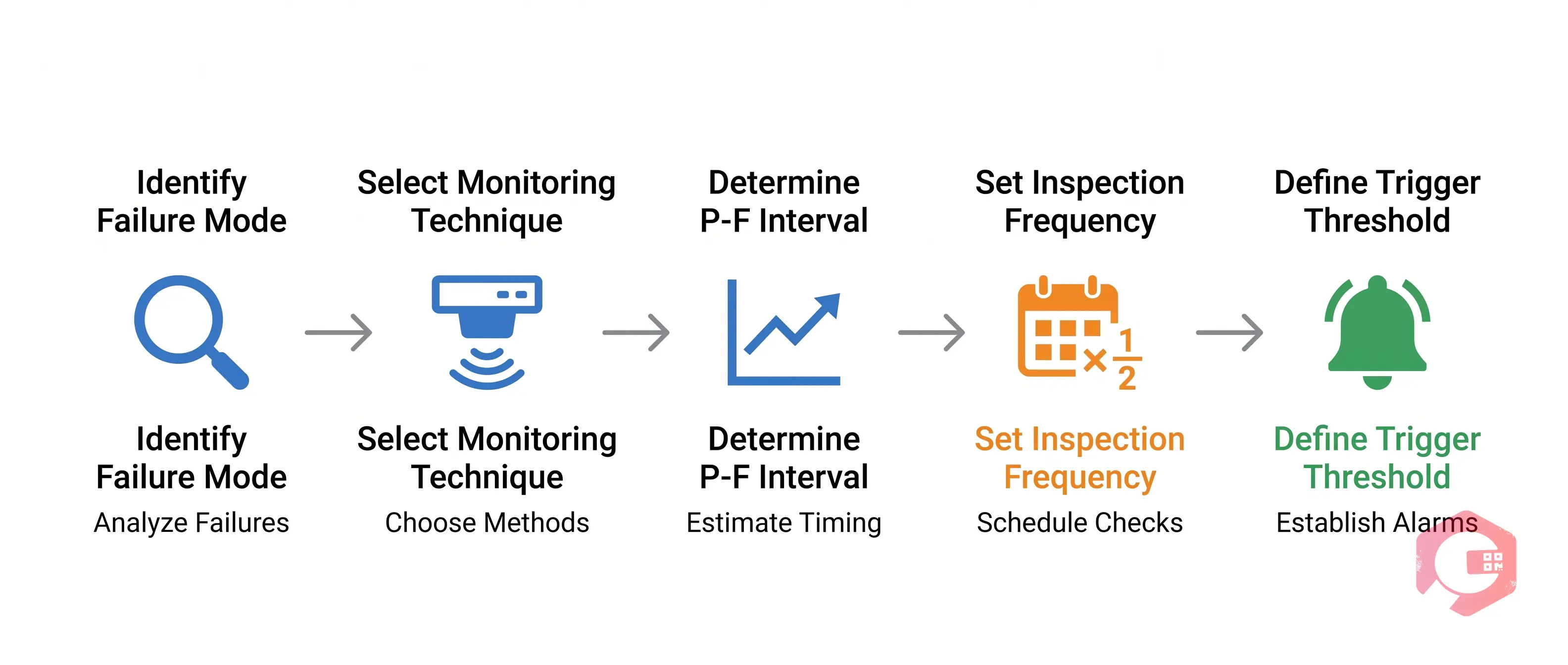
Setting a CBM interval is a deliberate, evidence-based process. Here are the five steps that maintenance engineers use in practice.
Start with a specific failure mode for the asset — not just "the pump fails" but "the pump bearing fails due to fatigue." Each failure mode has its own P-F characteristics. Use historical maintenance records, failure mode and effects analysis (FMEA), or RCM analysis to define the failure modes you are targeting. Trying to build a CBM program without this step leads to unfocused monitoring and missed failures.
For each failure mode, choose the monitoring technique that detects it earliest and most reliably. Bearing fatigue responds well to vibration analysis. Electrical insulation degradation shows up in partial discharge testing. Gear wear shows up in oil debris analysis. The technique you choose determines where on the P-F curve you will be monitoring — and therefore how long your P-F interval is.
The P-F interval is not a fixed number — it varies by asset type, operating conditions, and failure mode. To estimate it:
This is the core rule of P-F interval-based scheduling. If your P-F interval is 8 weeks, inspect every 4 weeks. If it is 30 days, inspect every 15 days. Inspecting at half the P-F interval ensures that even in the worst case — where you just missed a detection in the previous inspection — you will still catch the degradation before functional failure.
This rule has a name: the P-F interval halving rule. It is the single most important principle in setting defensible CBM frequencies. For high-criticality assets where failure consequences are severe, some engineers inspect at one-third of the P-F interval to add an extra buffer.
Inspecting is only half the task. You also need a defined threshold — a condition reading level — that automatically triggers a corrective work order. Without a threshold, technicians make judgment calls on every reading, which introduces inconsistency. The threshold should be set between Point P (first detection) and Point F (failure) — ideally closer to P to give maximum lead time for planning the repair.

Different techniques detect degradation at different distances from Point F. Understanding where each technique sits on the P-F curve helps you select the one that gives the most maintenance lead time for a given failure mode.
Setting CBM intervals manually works for a small number of assets, but as your program scales, managing hundreds of assets with individual P-F intervals becomes unworkable without software. A preventive and condition-based maintenance system automates the entire workflow.
Here is what that looks like in Cryotos:
Even experienced maintenance teams make these errors when setting up a CBM program around the P-F curve.
The P-F interval is the amount of time between the first detectable sign of a developing failure (Point P) and the point where the asset actually fails to do its job (Point F). It defines the window you have to detect, diagnose, and fix the problem before it becomes a breakdown.
The standard approach is to inspect at half the P-F interval. If your P-F interval is 6 weeks, schedule your condition monitoring inspection every 3 weeks. This ensures that even in the worst case — where you just missed the detection point in the previous inspection — you still have time to act before functional failure.
Not always. CBM is highly effective for failure modes that show detectable degradation signals — most mechanical, electrical, and fluid-system failures do. But some failure modes are random or have P-F intervals too short to monitor effectively. For those, time-based or run-to-failure strategies are still appropriate. A good maintenance program uses CBM where it makes sense and time-based maintenance where it doesn't.
The most common sensors used in CBM programs include vibration sensors (accelerometers), temperature sensors, current and power monitors, oil quality sensors, pressure transducers, and ultrasonic sensors. The right sensor depends on the failure mode you are targeting. IoT-connected sensors that feed data directly into your CMMS allow for real-time P-F monitoring without manual inspections.
A correctly set interval means you are catching failures at Point P consistently — before they reach functional failure — while not over-inspecting assets that are in good condition. Review your interval by tracking how often inspections find actual degradation versus clean readings. If nearly every inspection is clean, your interval may be too short. If you are regularly finding assets close to failure, your interval is too long.
The P-F curve gives maintenance teams a scientific basis for setting CBM intervals that are neither too frequent nor too late. By identifying the right monitoring technique for each failure mode, estimating the P-F interval from real data, and setting your inspection frequency at half that interval, you turn condition monitoring from a vague best practice into a precise, defensible schedule.
Cryotos makes this practical at scale. With IoT-driven threshold alerts, dynamic PM scheduling, and real-time asset condition tracking, Cryotos gives your team everything it needs to run a condition-based maintenance program that actually reduces failures — not just monitors them. Book a demo today and see how your team can put the P-F curve to work.


Cryotos AI predicts failures, automates work orders, and simplifies maintenance—before problems slow you down.