
Remaining useful life (RUL) is the estimated amount of operating time — hours, cycles, mileage, or calendar days — that an asset can keep running before it fails or drops below an acceptable performance level. Predictive models calculate remaining useful life using one of five approaches: physics-of-failure equations, statistical distributions, machine learning, degradation-curve extrapolation, or a hybrid blend of all three. Each approach fits a different mix of failure-mode knowledge and available sensor history.
Key Takeaways
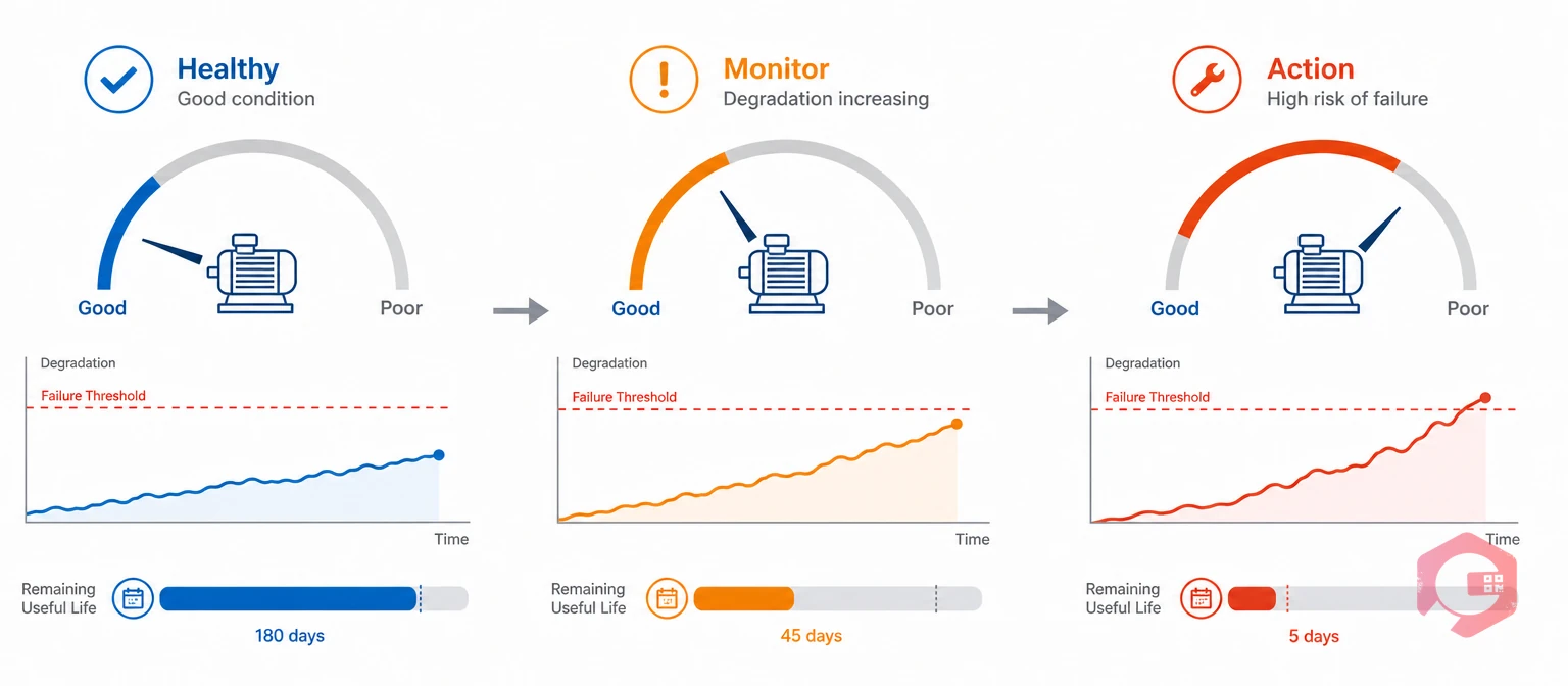
Remaining useful life (RUL) is the predicted operating time left on an asset before it reaches a defined failure point. That failure point might be a hard stop, like a bearing seizing or a belt snapping. Or it might be a soft one, like output dropping below a set percentage. Either way, RUL gives a maintenance team a number they can plan around instead of a guess.
A fixed replacement interval assumes every unit of the same type wears out on the same schedule. Remaining useful life rejects that assumption. It gets recalculated as new vibration readings, temperature trends, or run-hour totals come in. Two identical pumps installed on the same day can carry very different RUL estimates once they run under different loads.
For maintenance managers, RUL turns raw sensor data into a scheduling decision: fix it now, order the part today, or run the asset one more shift. Skip a structured RUL process and most teams land in one of two traps. They replace parts too early and waste budget, or they run parts too late and eat an unplanned failure.
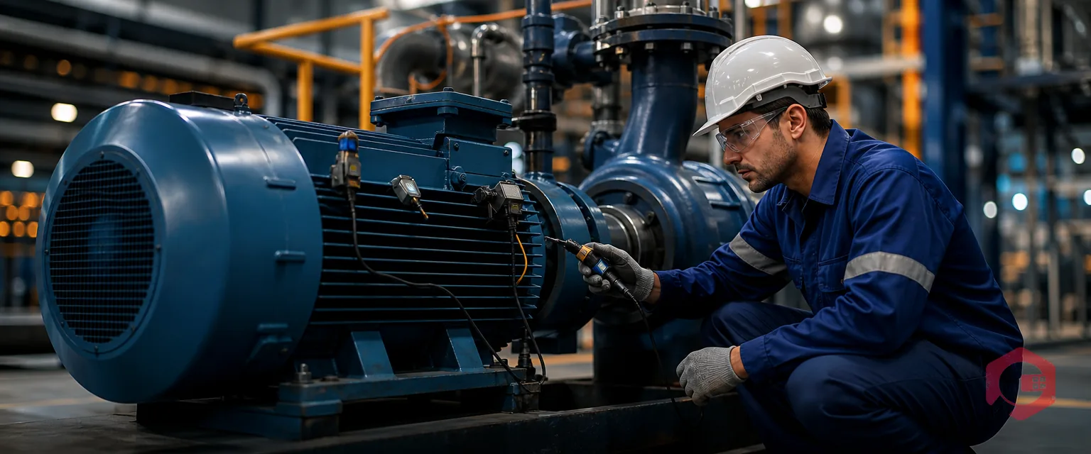
Picture a conveyor motor with a vibration sensor attached. Under normal conditions, the sensor reads 2 mm/s. Over three weeks, the reading climbs steadily to 4.5 mm/s. The failure threshold for that motor class is 6 mm/s. A simple trend model can look at that climb rate and estimate the motor has roughly 18 days of remaining useful life before it crosses the line. That single number is what lets a planner slot the repair into next week's maintenance window instead of waiting for a breakdown.
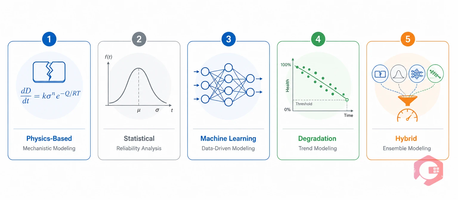
RUL is never produced by one universal formula. Teams pick from five modeling families, based on how much failure history and condition data exists for a given asset class.
The Five-Model RUL Stack:
A physics-of-failure model is an engineering equation that projects a known wear mechanism forward to its failure point. It starts from something the team already understands — fatigue crack growth, bearing wear, insulation breakdown — and uses a measured stressor like load, temperature, or vibration amplitude to run the projection.
These models work best when the failure mode is well understood and stays consistent across units. Rotating equipment bearings and structural fatigue in fixed-cycle machinery are common fits. A physics model needs less historical failure data than machine learning, since the underlying wear pattern is already known. It does lose accuracy fast, though, when a unit hits a stressor the equation never accounted for — a sudden overload, for example.
Where failure mechanisms are less predictable, teams turn to statistical distributions fitted to historical time-to-failure data. The most common choice is the Weibull distribution, along with exponential and log-normal models. A statistical reliability model is a probability curve built from past failure records, not a single fixed date. It might say there's a 70% chance a component survives another 400 operating hours, rather than naming one exact day.
Mean Time Between Failures and failure-rate calculations feed directly into this model class. The NIST Engineering Statistics Handbook covers the Weibull and exponential distributions used here in more depth, including how to fit them to a real dataset.
When a team has enough historical run-to-failure data, machine learning steps in. Regression models, random forests, and gradient-boosted trees learn the link between raw sensor readings and remaining life straight from the data. No physics equation is required.
For time-series-heavy condition data — vibration spectra, current draw, thermal trends — recurrent neural networks, LSTMs, and temporal convolutional networks are becoming common. They track how a degradation signature changes over time, not just its current value. That matters most for equipment with slow, compounding wear, where today's reading alone doesn't tell the full story.
Degradation-curve extrapolation is a trend line fit to a single condition reading, projected forward to a defined failure threshold. It's often the first method a team can deploy, because it needs less historical data than machine learning. Common inputs include vibration RMS, oil particle count, and insulation resistance.
The tradeoff is sensitivity. A single spike in vibration from a temporary load change, or one noisy sensor reading, can throw off the projected failure date. Teams that rely on this method often smooth the data first, or cross-check a sudden shift against a maintenance log before trusting the new number.
In practice, the most reliable RUL estimates blend more than one approach. A physics-based model sets the expected shape of the decline. Statistical distributions add the uncertainty range around it. Machine learning then corrects the estimate using real sensor drift picked up along the way.
Ensemble methods combine several model outputs and weight them by how accurate each one has been for that asset class in the past. Most teams running a mature predictive maintenance program end up here. No single model's blind spot gets to drive the final maintenance call on its own.
A predictive model rarely hands back one number with full certainty. A well-built RUL model returns a range — a median estimate of 45 days, say, with a 90% confidence interval running from 30 to 65 days.
Teams that look only at the median number, and skip the width of that range, tend to make one of two mistakes. Either they trust an early estimate built on thin data too much, or they under-react to a tightening window even as more data confirms the trend is real and getting close.
A widening confidence interval usually means the model hasn't seen enough data yet. It can also mean the asset's operating conditions have become less predictable — a change in load, for instance. A narrowing interval, especially one narrowing toward a shorter RUL, is the strongest signal a team gets that a failure is on schedule. That's the point where scheduling the repair stops being optional and starts being urgent.
Confidence intervals turn a raw model output into a decision a manager can defend, instead of a guess dressed up as data.
Each of the five modeling approaches trades off differently on data needs, setup cost, and accuracy. The table below breaks down where each one fits best.
| Model Type | Data Required | Best Fit | Main Limitation |
|---|---|---|---|
| Physics-of-Failure | Known degradation mechanism, stressor readings | Bearings, structural fatigue, well-understood failure modes | Weak on unmodeled stressors |
| Statistical / Reliability | Historical time-to-failure records | Fleet-level probability estimates, MTBF-driven planning | Returns a probability range, not a precise date |
| Machine Learning | Large run-to-failure datasets, sensor history | Complex, non-linear degradation patterns | Needs a lot of historical data to train well |
| Degradation-Curve | A single trending condition reading | Early-stage predictive programs, quick setup | Sensitive to noise and sudden condition changes |
| Hybrid / Ensemble | A combination of the above | Mature programs seeking the most reliable estimate | Higher setup and upkeep effort |
Most maintenance teams start with degradation-curve extrapolation, since it needs the least historical data. They move toward statistical and machine learning models once their failure history builds up inside a Computerized Maintenance Management System.
See how a shrinking RUL window affects your repair timelines with the MTTR calculator. It's a quick way to check whether your current repair turnaround can absorb a compressed failure window.
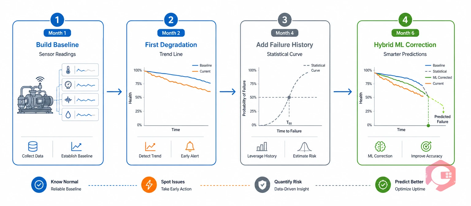
An RUL program looks different on paper than it does on a real fleet. Here's how it typically plays out for a plant running a set of air compressors.
The team installs vibration and temperature sensors on ten compressors. For the first month, there's no RUL model running yet — just raw readings feeding into an asset record. This step matters more than it looks. Without a clean baseline, any later model is just guessing at what "normal" looks like for that specific machine.
By month two, a clear trend shows up on Compressor 6. Vibration has climbed from 1.8 mm/s to 3.1 mm/s over four weeks. A simple degradation-curve model projects the reading will cross the 5 mm/s failure threshold in about 25 days. That's the first usable remaining useful life estimate for that machine.
By month four, two other compressors in the fleet have failed, and their pre-failure sensor data is now logged. A statistical model can use those two data points, alongside manufacturer reliability data, to build a rough survival curve for the whole compressor class. The RUL estimate for Compressor 6 tightens from a wide range to a narrower one, because the model now has real failure data to check its projection against.
Once enough run-to-failure cycles exist across the fleet, the team layers in a machine learning correction on top of the statistical baseline. The hybrid estimate catches a subtle pattern the simpler models missed: compressors running above a certain ambient temperature fail sooner than the base model predicted. That single insight resets maintenance priorities for three other machines in the fleet, well before any of them show an obvious warning sign.
Every RUL model, no matter which type, depends on the same underlying inputs: steady condition data, complete failure history, and reliability metrics tracked the same way over time. Cryotos builds that data foundation directly into the CMMS.
Cryotos connects to vibration sensors, temperature probes, current sensors, and other IoT devices via SCADA, PLC, and edge integrations, streaming real-time condition readings straight into the asset record. Without steady condition data, a model can only estimate from calendar time, not real wear.
Every work order, breakdown, and repair against an asset logs against that asset's record. That builds the run-to-failure history that statistical and machine learning models need in order to train. The longer an asset runs inside Cryotos, the more accurate the failure-time data available to any predictive model built on top of it.
Rather than fixed calendar intervals, Cryotos supports dynamic PM triggers tied to usage and condition-based maintenance thresholds. As a predicted RUL window shortens, PM tasks reschedule on their own, instead of waiting for the next calendar-based service date.
Cryotos calculates Mean Time Between Failures (MTBF), Mean Time To Repair, and failure rate automatically from work order and downtime data. These are the same reliability metrics that feed statistical RUL models.
The Cryotos BI dashboard surfaces degradation trends across assets and equipment classes. It can flag a compressor whose vibration trend is climbing faster than its class average — an early, visual signal before a full model output is even needed.
When a monitored value crosses a defined threshold, Cryotos automatically generates a corrective or inspection work order. It's pre-linked to the asset and routed to the right technician, closing the gap between a shrinking RUL estimate and an actual maintenance action.
Push notifications, SMS, and email escalations notify managers and technicians as an asset's estimated remaining life drops into a critical range. A narrowing window gets acted on right away, instead of getting discovered after the fact.
Cryotos integrations with SAP and Microsoft Dynamics 365, combined with its inventory management module, let teams check parts availability against a predicted failure window. That way, the corrective work order isn't stuck waiting on a part that should have been ordered weeks earlier.
Maintenance teams using Cryotos have reported up to 30% reduction in unplanned downtime and 25% faster repair turnaround as RUL-driven scheduling replaces guesswork with structured data.
An accurate RUL estimate changes what a maintenance team does next, not just what they know. A few patterns show up again and again at facilities that put RUL into practice.
Teams replace a component close to the true end of its useful life, instead of on a fixed calendar schedule. That captures more of the part's service life while still staying ahead of the unplanned failure window.
Procurement times parts orders against predicted failure dates instead of carrying excess inventory for every asset as a hedge against unknown timing. That frees up working capital that would otherwise sit on a warehouse shelf.
Aggregated RUL data across an asset class gives leadership a forward-looking view of which machines are nearing end-of-life. That supports budget decisions months or years ahead of a forced, unplanned replacement.
When dozens or hundreds of assets each carry an RUL estimate, teams can rank backlog by urgency and consequence, rather than working strictly first-in-first-out. Limited technician hours go to the assets closest to failure first.
Because RUL-driven scheduling steps in before the failure threshold is reached, downtime shifts from reactive to planned. That reduces production loss and the safety exposure that comes with a sudden equipment failure.
Most facilities that track this shift find the biggest gain isn't model accuracy on its own. It's how much sooner a shrinking window gets escalated to someone who can act on it. The Society for Maintenance and Reliability Professionals lists this kind of proactive scheduling shift among the core signs of a mature reliability program. The broader field of prognostics exists for exactly this reason. Its whole goal is a longer, more reliable lead time before failure.
A few terms come up again and again in RUL work. Here's what each one means in plain terms.
Keep these five terms handy. They show up in almost every RUL report, regardless of which model built it.
Most RUL programs don't fail because the math is wrong. They fail because of a few small habits that quietly undo good data. Here are the mistakes that show up most often.
A short gap in sensor data — a network outage, a sensor swap, a missed reading — can throw off a trend line more than most teams expect. The model has to guess at what happened during the gap. That guess can shift the whole projection by days or weeks. Most mature programs treat a data gap as a flag on its own, not just a missing number to fill in later.
Remaining useful life predicts the time left on one specific asset, based on its actual condition data. Mean Time Between Failures is a fleet-level average pulled from historical failure records. RUL answers "how long does this exact pump have left," while MTBF answers "how often does this class of pump typically fail."
Degradation-curve extrapolation can start with just a few weeks of trending condition data on a single asset. Machine learning models usually need dozens of complete run-to-failure cycles across similar assets before the predictions become dependable. Most teams start with the simpler method and add data-driven models as their failure history builds.
No single RUL model returns a guaranteed number. Every credible model returns an estimate with a confidence range around it. The goal isn't a perfect prediction — it's a defensible, data-backed window that's tight enough to plan a repair around with confidence.
Most small teams start with degradation-curve extrapolation on their highest-criticality assets. It needs the least historical data and can run on condition readings the team is likely already collecting. Statistical and machine learning models become practical once failure history builds up inside a CMMS.
No. RUL prediction usually layers on top of preventive maintenance rather than replacing it outright. Many facilities keep baseline PM tasks for routine servicing, then use RUL estimates to catch the specific assets whose actual wear is running ahead of, or behind, that baseline schedule.
An RUL estimate should be recalculated every time meaningful new condition data arrives, not on a fixed schedule. For assets under continuous IoT monitoring, that can mean the estimate updates daily, or even hourly, as fresh sensor readings come in.
A disagreement between models is a useful signal on its own, not just a problem to resolve. It usually means one model is missing a stressor the other one is picking up on. Many hybrid programs treat a wide split between model outputs as a reason to flag the asset for a closer manual inspection, rather than simply averaging the two numbers together.
No. Total lifespan is how long an asset lasts from installation to final retirement. Remaining useful life is a moving number that changes throughout that lifespan. An asset can have a long total lifespan overall, but a short remaining useful life right now if it's running under heavy stress.
Estimating remaining useful life well isn't about picking the one "correct" model. It's about matching the right model to the data a team actually has, then feeding that model better data over time. A young predictive program and a mature one can use the exact same five-model stack — they just sit at different points along it.
Turning a shrinking remaining useful life estimate into a scheduled work order, instead of an unplanned failure, starts with having the right data foundation in place. Schedule a free demo to see how Cryotos connects condition monitoring, failure history, and reliability analytics into one system that predictive models can actually work from.
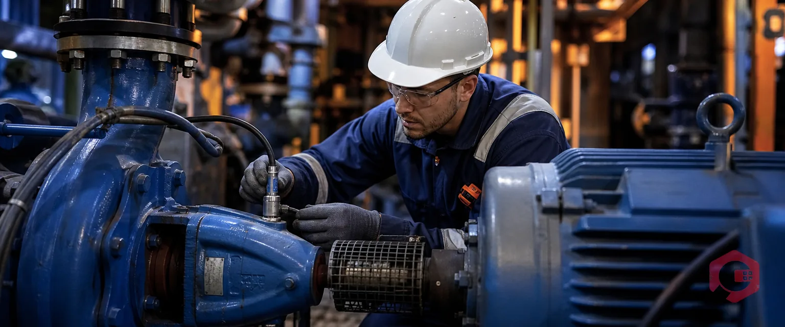


Cryotos AI predicts failures, automates work orders, and simplifies maintenance—before problems slow you down.