Spare parts demand variance in high-mix manufacturing is the swing in parts usage caused by constantly changing products, batch sizes, and changeovers. It is the reason a part sits untouched for weeks, then runs out in one shift.
Averages and calendar-based reorder points miss this pattern, because what a machine consumes depends on what it ran last week. A Computerized Maintenance Management System links each parts issue to an asset, a work order, and a production change, which makes the pattern visible. This guide covers what drives the swings, how to measure them, and which stocking rule fits each type.
Key Takeaways
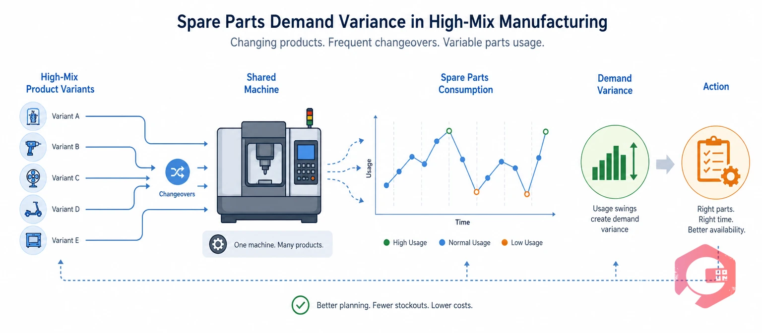
High-mix manufacturing is a production model that builds many product variants in small batches on shared equipment. Each switch between variants changes how hard a machine works, and that is why spare parts demand variance runs higher here than on single-product lines.
A packaging line that runs one product for a month wears its parts at a steady pace. A line that runs forty variants in a month does not. Material, speed, and tooling change every few hours, and parts wear to match.
Asset management guidance such as ISO 55000 asks organizations to tie stock decisions to risk and value. SMRP metrics give maintenance teams shared definitions for inventory and reliability. Both point to the same first step: understand why demand moves before you set a stock level.
Variance is not a data problem to smooth away. It is a signal about how the plant runs.
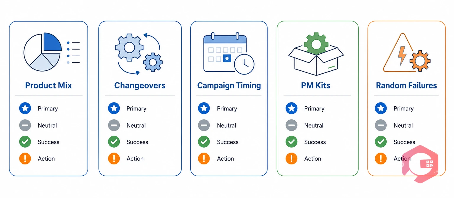
Most spare parts demand variance in a high-mix plant traces back to five drivers, and only one of them is random. The matrix shows each driver, what it does to parts usage, and where to find it in your data.
| Driver | What changes on the floor | Effect on parts usage | Example parts | Where to see it |
|---|---|---|---|---|
| Product mix shifts | Variants load machines differently through material, speed, and weight | Wear follows the product, not the calendar | Cutting tools, nozzles, wear plates | Production schedule by asset |
| Changeover frequency | Tooling, dies, and format parts are swapped often | Usage rises with each changeover | Clamps, sensors, seals, change parts | Changeover log |
| Batch and campaign timing | Similar products are grouped into campaigns | Parts wear in clusters, then go quiet | Belts, blades, filters | Weekly run plan |
| Calendar PM kits | Planned tasks fall on the same dates | Predictable spikes in PM weeks | Filters, lubricants, gaskets | PM schedule |
| Random failures | Breakdowns with no clear pattern | Unpredictable, often one-off | Bearings, motors, drives | Corrective work orders |
The first four drivers can be forecast from the plan. Only the fifth needs statistics, yet many maintenance teams treat all five as random and hold stock for events the schedule already predicts. Manufacturing maintenance software ties work orders to production assets, which exposes these drivers faster.
Want to see what a stockout costs your line? Try the unplanned downtime calculator and use the result to size your buffers.
The coefficient of variation (CV) is the standard deviation of usage divided by its mean. As a rough guide, a CV near 0.2 means usage is steady, and a CV above 1.0 means usage swings by more than its own average. This overview of the coefficient of variation shows the formula.
Compare the two CV values for each part. If the CV falls sharply after normalizing, the variance is mix-driven, and the production plan can forecast it. If the CV stays high, the spare parts demand variance is random and needs a buffer.
Parts used in only a few months each year need one more check. Count the share of months with any usage, because a CV calculated on mostly zero data can mislead.
This illustrative example follows a clamp seal on a filling line that runs many product variants. Six months of issues look random at first glance.
| Month | Changeovers | Units used | Units per changeover |
|---|---|---|---|
| Month 1 | 20 | 4 | 0.20 |
| Month 2 | 5 | 1 | 0.20 |
| Month 3 | 45 | 9 | 0.20 |
| Month 4 | 10 | 2 | 0.20 |
| Month 5 | 5 | 1 | 0.20 |
| Month 6 | 35 | 7 | 0.20 |
| Average | 20 | 4.0 | 0.20 |
Usage ranges from 1 to 9 units a month, with a mean of 4 and a sample standard deviation of about 3.3, so the CV is about 0.84. Yet every month the plant used 0.2 units per changeover. The variance sits in the changeover count, not in the part.
Next month's plan shows 30 changeovers, so expected demand is 6 units. The forecast now follows the schedule, and only a small gap is left for safety stock to cover.
Each source of spare parts demand variance calls for a different stocking rule. Match the rule to the source, and you avoid paying for safety stock the schedule already makes unnecessary.
| Variance source | Signal in your data | Stocking rule | Review trigger |
|---|---|---|---|
| Mix-driven | CV falls after normalizing by changeovers or hours | Forecast from the production plan and stock for the next one or two planning cycles | New product launch or schedule change |
| Calendar-driven PM kits | Usage lines up with PM dates | Reserve parts against scheduled work orders and kit them before the PM week | PM interval change |
| Random failure, frequent | High CV, with usage in most months | Reorder point with safety stock over the supplier lead time | Quarterly service-level review |
| Random failure, rare and critical | Zero in most months, but line-stopping if missing | Hold one insurance spare and share it across sites where possible | Annual criticality review |
| Project or one-off | A single large issue | Buy to order and keep it out of the average | Project close |
Plan reservations from the calendar in your preventive maintenance software, so PM kits never compete with breakdown stock. For random failures, use failure history such as mean time between failures to judge how often a part will be needed.
Safety stock is the extra inventory held to cover swings in demand while a supplier order is on the way. For parts with steady, bell-shaped usage, a common formula applies, and this explanation of safety stock covers its background.
Safety stock equals the service-level z-value, times the standard deviation of demand per period, times the square root of the lead time in periods. A 95% service level uses a z-value of about 1.645.
The service level stays at 95%, and the buffer falls by four units. Multiply that across hundreds of mix-driven parts, and the freed cash adds up.
Two limits apply. The bell-curve formula breaks down for parts used in only a few months a year, so use a lead-time demand probability or an insurance-spare rule for them. Lead-time variation also needs its own allowance. Set the resulting minimum and maximum levels with alerts in inventory management, so the rule runs without manual checks.
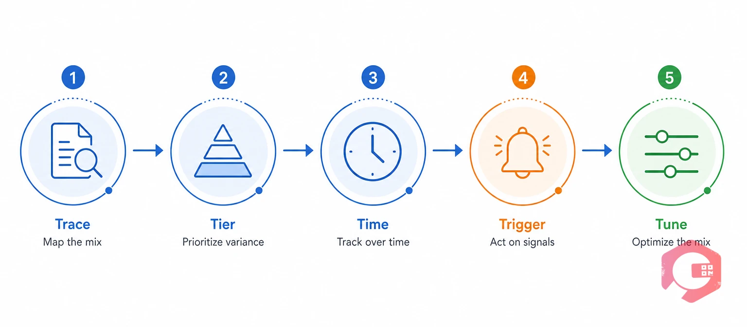
Maintenance teams in high-mix plants can manage spare parts demand variance with a five-step routine that fits into the weekly planning meeting.
The Mix-Variance Control Framework:
Most facilities already hold the raw data for the Trace step. The routine depends on consistency, not on new tools.
The most common mistakes come from treating spare parts demand variance as noise instead of a signal. Most high-mix plants repeat the same five.
Fixing these habits costs little and often frees more cash than any new forecasting tool.
A 90-day start on one line keeps the scope small and gives operations a clear result on spare parts demand variance.
Compare stockout days and emergency purchases with the previous quarter. Early results make the case for extending the routine to the next line.
Cryotos keeps parts, assets, work orders, and PM schedules in one mobile-first platform, so the Trace step happens as a side effect of normal work. Its spare parts inventory software gives the stock view that spare parts demand variance rules depend on.
Maintenance teams using Cryotos have reported up to 30% reduction in unplanned downtime and 25% faster repair turnaround. Cryotos does not run demand forecasts on its own. It supplies the clean usage data that a driver-based forecast needs.
Product mix shifts, frequent changeovers, campaign scheduling, clustered PM kits, and random breakdowns cause most of it. The first four follow the production plan, so they can be forecast.
Divide the standard deviation of monthly or weekly usage by its mean to get the coefficient of variation. Then divide usage by a driver, such as changeovers, and recalculate to see how much variance the driver explains.
Yes, if part of the spare parts demand variance is explainable. Forecasting that part from the production schedule lowers the error that safety stock must cover, so the buffer can shrink at the same service level.
A moving average assumes the recent past predicts the near future. In a high-mix plant, the next batch can wear parts differently from the last one, so the average lags behind the schedule.
Start with parts on the constraint machine, high-spend parts, and parts with repeated emergency purchases. These carry the highest cost of getting the stock level wrong.
Steady lines are easy to stock, and high-mix lines are not, until the stock rule follows the schedule. Schedule a free demo to see how Cryotos links parts, work orders, and production changes in one view.


Cryotos AI predicts failures, automates work orders, and simplifies maintenance—before problems slow you down.