Weibull analysis for maintenance is a statistical method that uses past failure data to predict when equipment will fail next. Named after Swedish engineer Waloddi Weibull, it gives maintenance teams a full failure probability curve — not just a single average. Teams can then set replacement intervals based on actual risk, not guesswork. According to Reliabilityweb, it is the tool of choice for most reliability engineers working with age-to-failure data.
For teams running a Computerized Maintenance Management Software, Weibull provides a statistical backbone for data-driven replacement decisions. It cuts emergency repair costs and removes guesswork from the schedule.
Key Takeaways

Weibull analysis is a statistical method that predicts failure timing from historical failure data. Unlike methods that assume a fixed failure rate, it accounts for the fact that failure behaviour changes with age. This makes it far more accurate for maintenance planning than a fixed manufacturer-recommended interval.
The analysis uses two primary parameters — shape (β) and scale (η) — plotted on a log-log scale. The slope and position of the resulting line tell maintenance engineers what failure mode is active and when replacement should be scheduled.
As the Weibull distribution entry on Wikipedia notes, the distribution has been validated across industrial equipment, electronics, and civil infrastructure. For maintenance teams, this means one method works across pumps, motors, bearings, conveyor systems, and HVAC units.
Swedish mathematician Waloddi Weibull introduced it in 1939 to model material strength. By the 1970s, reliability engineers had adopted it as the standard tool for analysing time-to-failure data. It fits roughly 85–95% of all life data found in field conditions — which is why it remains the default choice.
Most practical Weibull analysis uses two parameters. Advanced cases — where equipment has a guaranteed failure-free period — add a third. Knowing what each parameter means is the difference between misreading your data and acting on it correctly.
The beta parameter is the most important Weibull number — it identifies your asset's failure mode. A beta below 1.0 means early-life failures where defects are weeded out over time. A beta near 1.0 means random failures with no age relationship. A beta above 1.0 means wear-out — failures that increase as the asset gets older. Most rotating mechanical components in wear-out mode show beta values between 1.5 and 5.0.
The eta parameter is the characteristic life — the age by which 63.2% of similar assets will have failed. This 63.2% relationship holds regardless of the beta value, making eta the single reference point for comparing asset lifespans across your fleet. If your pump's eta is 15,000 hours, you know the median failure window — and can set replacement intervals well before that point.
The gamma parameter applies only in 3-parameter Weibull models. It represents a guaranteed minimum failure-free period — the time before which no failures are expected. This applies to components with a definite break-in window or assets where warranty data shows zero early failures. Most CMMS-driven maintenance teams work with the 2-parameter model; gamma is set to zero by default.
The bathtub curve is a three-phase model showing how asset failure rate changes with age, mapped onto Weibull beta values. Knowing which phase an asset is in determines the correct maintenance strategy — and prevents wasting PM budget on the wrong response.
Most mechanical assets maintenance teams manage will be in the wear-out phase. A beta between 2 and 4 is the most common profile for rotating components — which is exactly where preventive replacement is both justified and cost-effective.
Running a Weibull analysis does not require a statistics degree. With a CMMS that captures structured failure data, most maintenance engineers can complete the process in Excel or dedicated reliability software like ReliaSoft Weibull++ or Minitab.
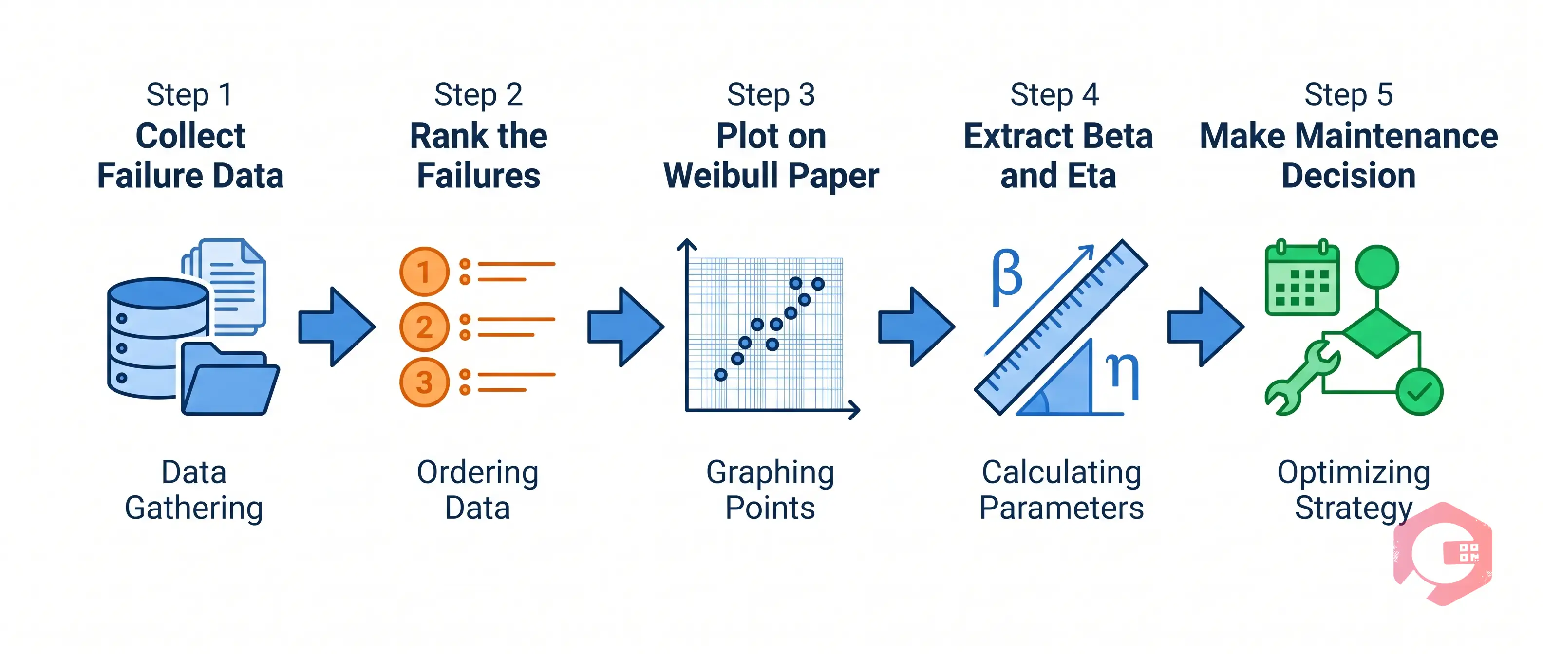
Gather time-to-failure records for the asset or asset class. You need a minimum of 5–10 actual failure events — not maintenance actions, but confirmed failures. Each record must include the failure date, asset ID, failure mode, and time in service at failure. Your CMMS work order history is the primary source. If an asset was still running when data collection ended, record it as a suspension (censored data). This keeps the analysis valid without throwing away useful uptime information.
Sort failures in order and assign a median rank to each using: Median Rank = (i − 0.3) / (n + 0.4). Here i is the rank order and n is the total number of data points. This rank is the cumulative failure probability for each observed failure time. Most reliability software handles this step automatically.
Plot failure time on the x-axis and cumulative failure probability on the y-axis using a log-log scale. A straight line through the data points confirms a good Weibull fit. Curvature suggests a 3-parameter model or a mixed failure mode that needs to be separated before re-plotting.
Read the slope of the fitted line (beta) and the x-axis value at which the cumulative probability equals 63.2% (eta). Software calculates both automatically. Beta tells you the failure mode. Eta tells you the asset's natural lifespan under current operating conditions.
Use beta and eta to set a replacement interval at a failure probability your team accepts — usually 10–20% cumulative probability. If a bearing has a beta of 2.5 and an eta of 12,000 hours, plan replacement at roughly 8,000–9,000 hours. Adjust PM task frequencies, spare parts stock, and work order triggers accordingly.
Use our free MTBF calculator to cross-reference Weibull-derived life estimates with your fleet's observed between-failure intervals before finalising any PM schedule changes.
Weibull analysis answers "when will this fail?" — but FMEA (Failure Mode and Effects Analysis) answers "what fails, how, and with what consequence?" Using both together gives maintenance teams a full picture: failure probability over time, ranked by business impact. This two-tool approach is a core principle of ISO 55000, which requires asset decisions to be grounded in both risk and reliability data.
In a reliability-centered maintenance programme, Weibull feeds directly into the RCM decision logic. When beta is clearly above 1, RCM recommends a scheduled replacement task — and Weibull tells you the exact interval. When beta is near 1, RCM directs you toward condition-based monitoring — and Weibull confirms that time-based PM adds no value for that mode.
Teams that link FMEA failure modes to Weibull-derived intervals get tighter alignment between PM frequency and actual asset risk. This cuts both over-maintenance waste and unexpected failures from under-maintenance.
As noted in Relyence's introduction to Weibull analysis, results depend heavily on data quality and correct interpretation. Most operations that struggle with Weibull make one of these five mistakes.

Weibull analysis is only as reliable as the failure data behind it. Maintenance teams using Cryotos have reported up to 30% reduction in unplanned downtime and 25% faster repair turnaround — in large part because Cryotos structures the exact failure capture process that Weibull depends on.
The Weibull Maintenance Decision Loop:
A minimum of 5–10 actual failure events gives you a workable result, but 20 or more data points produce significantly more reliable parameter estimates. If an individual asset has fewer than 5 failures in its history, combine records from identical assets running under the same conditions to build a statistically valid dataset before plotting.
MTBF gives you a single average time between failures. Weibull gives you a full probability curve — showing the spread and shape of failures around that average. For replacement planning, Weibull is far more actionable because it shows failure risk at any specific point in time, not just the mean. You can use our failure rate calculator to cross-check your Weibull-derived intervals against observed data.
Yes. Excel handles basic two-parameter Weibull analysis using median rank calculations and log-log plots. For larger datasets, mixed failure modes, or censored data, dedicated tools like ReliaSoft Weibull++, Minitab, or the open-source Reliability Workbench provide better automation and statistical rigour. Most operations start with Excel and move to specialist software as their data volumes grow.
A beta above 1 confirms wear-out failure mode — your asset's failure rate increases with age. This is the most common profile for rotating mechanical components like bearings, seals, and gearboxes, and it means time-based preventive replacement at a defined interval is fully justified. Weibull tells you exactly what that interval should be, based on your acceptable failure probability and the eta value for that component population.
In an RCM programme, Weibull validates the maintenance task type chosen for each failure mode. For wear-out failures (beta greater than 1), RCM prescribes scheduled replacement — and Weibull provides the exact interval. For random failures (beta near 1), RCM prescribes condition-based monitoring — and Weibull confirms that time-based PM adds no value for that mode. Together, the two methods cut both over-maintenance waste and unplanned breakdowns from under-maintenance.
Weibull analysis turns historical failure data into a clear, defensible maintenance schedule — but only when your data foundation is solid. Schedule a free demo to see how Cryotos structures failure capture, asset history, and IoT-connected monitoring so your reliability team always has the clean data Weibull demands.


Cryotos AI predicts failures, automates work orders, and simplifies maintenance—before problems slow you down.